Visualizing EIANN network structure

Note

🚧 Work in Progress: This documentation site is currently under construction. Content may change frequently.

In this tutorial, we will show some examples of what we can analyze about the internal structure of an EIANN network after we have applied our chosen learning algorithm and trained it.

import EIANN.EIANN as eiann
from EIANN import utils as ut
eiann.plot.update_plot_defaults()
root_dir = ut.get_project_root()
%load_ext autoreload
%autoreload 2

Show code cell output

Hide code cell output

The autoreload extension is already loaded. To reload it, use:
  %reload_ext autoreload

For convenience, we’ve packaged the code for loading the MNIST dataloaders into a separate function:

# 1. Loading the MNIST dataset
train_dataloader, val_dataloader, test_dataloader, data_generator = ut.get_MNIST_dataloaders()

Now we can load the network that was trained in the previous tutorial:

# Load network object from pickle file
network_name = "example_EI_network"
network = ut.load_network(path= f"{root_dir}/EIANN/saved_networks/mnist/{network_name}.pkl")

Loading network from '/Users/ag1880/github-repos/Milstein-Lab/EIANN/EIANN/saved_networks/mnist/example_EI_network.pkl'
Network successfully loaded from '/Users/ag1880/github-repos/Milstein-Lab/EIANN/EIANN/saved_networks/mnist/example_EI_network.pkl'

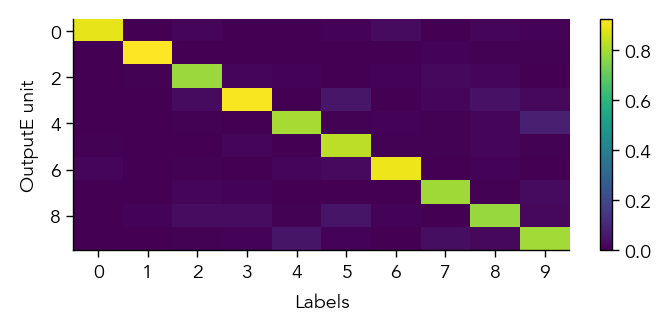
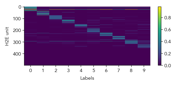
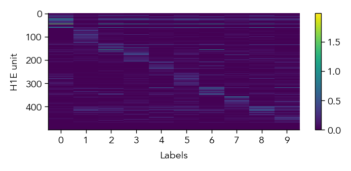
1. Analyze population activities

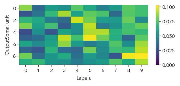
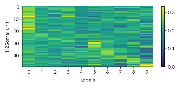
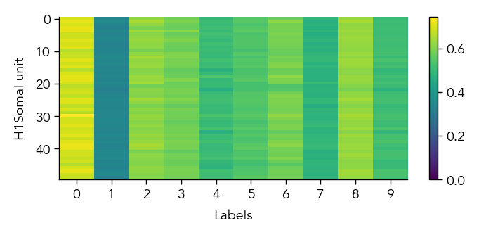
To get a first overview of how the network is representing different stimuli categories, we can plot the average activity of each unit in the network across the different stimulus categories (in this case MNIST digit labels). This gives us a sense of how selective units are to particular image categories and how distributed or sparse the representation is at the population level.

eiann.plot.plot_batch_accuracy(network, test_dataloader, population='all')

Batch accuracy = 94.69000244140625%

If our network has recurrent connections (such as in an EI network), we can also visualize the network temporal dynamics within each sample. This gives us a sense of how stable the network is, or if there are significant oscillations that might affect our learning algorithm. For example, if there are separate recurrent E and I populations we might generally expect some initial oscillations when we present a new stimulus, which should eventually equilibrate to a stable state (depending on the exact values/strength of the recurrent connections).

pop_dynamics_dict = ut.compute_test_activity_dynamics(network, test_dataloader, plot=True, normalize=False) # We will evaluate the network dynamics by presenting the test dataset and recording the neuron activity.
print(pop_dynamics_dict['H1E'].shape) # Since we are store the dynamics here, each population should have activity of shape (timesteps, data samples, neurons)

torch.Size([18, 10000, 500])

2. Analyze learned representations

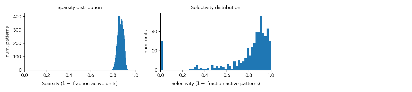
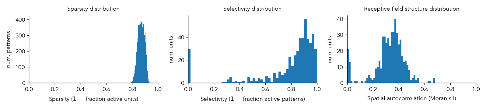
At the population level, we can quantify various aspects of the learned representation, such as the sparsity (how many neurons are active at any given time) and the individual selectivty (how selective each neuron is to a particular stimulus).

metrics_dict = ut.compute_representation_metrics(population=network.H1.E, dataloader=test_dataloader, plot=True)

If we want a more in-depth look at how individual neurons are behaving and which features of the input they have learned, we can generate a visualization of all the “receptive fields” for a given population. This is done through a function that optimizes an input image to maximally activate a given neuron in the network.

receptive_fields = ut.compute_maxact_receptive_fields(network.H1.E, test_dataloader=test_dataloader)
eiann.plot.plot_receptive_fields(receptive_fields, sort=True)

Optimizing receptive field images...

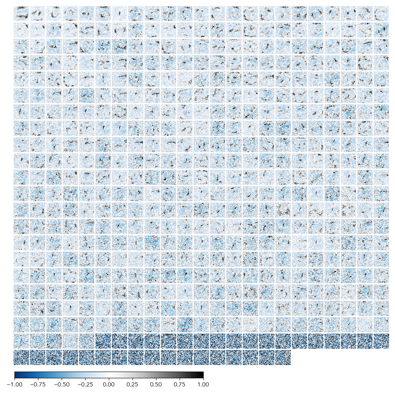
In this example, we can see that in the Excitatory cells of the first hidden layer (H1.E), most neurons have learned to form simple receptive fields that are similar to Gabor filters and sensitive to particular orientations and spatial frequencies within different regions of the image.

To compare this more quantitatively across different neural networks, we can quantify how ‘structured’ the receptive fields are by measuring their spatial autocorrelations using a metric called Morans I.

metrics_dict = ut.compute_representation_metrics(population=network.H1.E, dataloader=test_dataloader, receptive_fields=receptive_fields, plot=True)

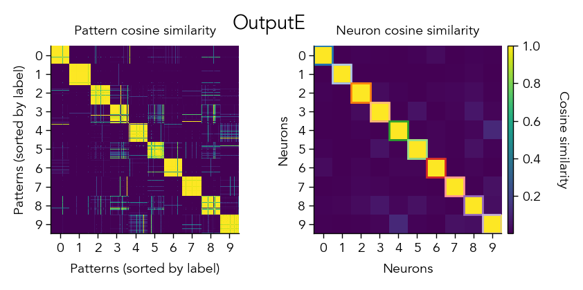
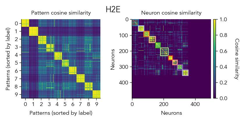
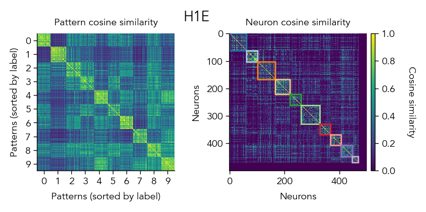
Another way to look at the learned representations is through a representational similarity analysis (RSA), where we can compare how similar the population representations are for different stimuli.

pop_activity_dict, pattern_labels, unit_labels_dict = ut.compute_test_activity(network, test_dataloader, class_average=False, sort=True)
pattern_similarity_matrix_dict, neuron_similarity_matrix_dict = ut.compute_representational_similarity_matrix(pop_activity_dict, pattern_labels, unit_labels_dict, population='E', plot=True)

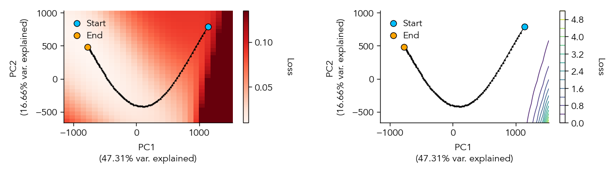
3. Analyze learning dynamics

If we set the option store_params=True during training, we can also visualize the trajectory through the weight space during training as the network descents the loss landscape towards a local minimum.

eiann.plot.plot_loss_landscape(test_dataloader, network, num_points=20, extension=0.1, vmax_scale=1.2)